and you want to achieve a -precision on the objective function , i.e., you want to obtain an estimate of such that .
Since is continuous, you cannot have access to all values when describes the constraints , but you can allow yourself multiples calls to the “oracle” in order to achieve this precision.
A naive way to do so is to consider a discretization of of precision , that is
and its counterpart in dimension .
It is easy to see that taking the minimizers of over satisfies the property as soon as is -Lipchitz.
So what’s the deal?
The issue is that the size of grows exponentially fast with the dimension .
In dimension 1, one needs to perform evaluations of , but in dimension , one needs !
This quantity gets prohibilitively large in a too fast manner: say you look at a very modest precision of , then in dimension , only 200 computations of are needed, whereas in dimension , you already need 200000000000000000000 evaluations (that’s 20 zeros).
This is known as the curse of dimensionality, a term introduced by (Bellman, Richard E., 1961) [Chapter V] for optimal control and (over)used since then in the optimization, statistics and machine learning communities (Donoho, David L, 2000).
Summary: we need to be (slightly) more clever.
1 Descent direction
Consider the class of algorithms of the form
how to “optimaly choose” the direction such that is closer to a minimum of ?
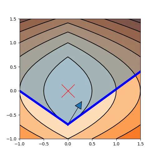
Definition 1
Let .
A descent direction of at is vector such that
Figure 1.Descent cone.
Observe that if is differentiable, this property is equivalent to .
The negative gradient is the direction of steepest descent at the point .
Proposition 2
Let be a differentiable function at .
Then, the problem
has a unique solution .
Proof
Let such that .
Consider the function defined by
The function is differentiable at and its derivative reads .
Denoting the angle between and , we have that .
Hence, minimizing is equivalent to finding the minimum of , that is for some .
Thus, we have
2 The gradient descent (GD) algorithm
Proposition 2 gives birth to what is known as the gradient descent algorithm or gradient descent method.
Algorithm 1.
Input: Initialization , step-size policy .
fordo
The choice of the step-sizes is crucial, and there is several way to do it.
Predetermined.
In this case, the sequence is chosen beforehand, either with a constant step size or with a given function of , , e.g., for some .
For some classes of optimization problem, it is possible to provide guarantees depending on the choice of .
Oracle.
This is the “optimal” descent that a gradient descent method can produce, defined by
Remark that this choice is only theoretical since it involves a new optimization problem that may be nonsolvable in closed form.
Backtracking rule.
Another time…
3 Rates of convegence
3.1 Means of convergence
In optimization, we consider several types of (worst-case) convergences:
Convergence in norms of the iterates.
Assuming that there exists a minimizer , the convergence in norms (for a given norm, typically the Euclidean one) looks at an -solution in the sense of
Note that there may be several minimizers, but we only consider one given minimzier.
Convergence to the set of minimizers.
Here, we look at the distance to any minimizer:
where is the set of minimizer.
Convergence in value (0-order).
Assuming that the infimum of the problem is given by , an -solution is given by
and assuming is a solution, this is the quantity .
First-order convergence.
If is differentiable, one can looks at the gradient of the iterates as
The idea is to use the first-order condition, and say that the more , the closer we are from a critical point of if is nonconvex, and closer from a global minima if is convex.
3.2 Rates versus complexity
To be more precise, we consider -rate below, there is an alternative definition (-convergence).
Sublinear rates.
We say that enjoys a sublinear rate if it has an upper bound written as a power function of , i.e. where and .
Typical examples are stochastic gradient descent enjoying a rate for convex functions or the gradient descent enjoying a rate for convex -smooth functions.
In term of complexity, if enjoys a rate, its complexity bound is .
For instance, the SGD for convex functions has complexity .
Linear rates.
We say that enjoys a linear rate if it has an upper bound written as an exponential function of , i.e. for and .
Note that typically, we don’t obtain directly the exponential function in proofs, but an even more precise one: that is directly bounded by .
In term of complexity, we have the bound .
Quadratic rates.
We say that enjoys a quadratic rate if it has an upper bound written as
for .
In terms of complexity, we have the bound : each iteration doubles the precision of the estimate!
Note that quadratic rates are a special case of a wider class known as superlinear convergence.
4 Explicit analysis of the gradient descent: ordinary least-squares
This part is heavily inspired from (Bach, Francis, 2021, chapter V).
Let , and .
The least-square estimator is defined by the problem
The objective is twice differentiable, its gradient reads
and its Hessian is constant on the whole space:
Note that there is at least one minimizer to the problem (1).
The first-order condition for a potential minimizer is given by
A necessary, and sufficient condition, to have exactly one minimizer is that is invertible.
The following lemma shows that, providing the knowledge of , the $t$-iterates of the gradient descent with fixed step-size is computable in closed-form.
Lemma 3
For all , we have
Proof
Using the expression of the gradient, we have for any minimizer
Substracting from both side gives
This identity is linear recursion, and unrolling it leads to the result.
4.1 Convergence in norm
We denote by the smallest eigenvalue of , its largest, and we let its condition number.
We have and .
Remark that the eigenvalues of are exactly given by where is an eigenvalue of .
Since all eigenvalues of are contained in , one also can bound any by
Suppose that there is multiple minimizers.
In this case, is not invertible and the smallest eigenvalue is equal to 0. Hence, there exists such that .
Choose a minimizer.
Using , we have
Hence, the method is not necessarly convergent, depending on the initialization.
The situation is different when we assume that there is a unique minimizer.
Proposition 4
Assume that (1) has a unique minimizer .
Then, the gradient descent iterates with constant step-size converges linearly in norm
Proof
Since there is a unique minimizer , we have .
Observe that (using a spectral norm bound)
Observe that is minimized for , and value is .
Indeed,
Hence,
Moreover, we have the following set of equivalence
This minima is achieved when the two curve and intersect.
Choice independant from the strong-convexity constant: It is possible to chose a smaller stepsize (hence slower) by taking the suboptimal value .
In this case, we get
In both cases, we obtained a linear (or geometric, or exponential depending on the community) rate
where or depending on the choice of the step-size.
It is possible to also speaks in term of iteration complexity.
Assuming the choice of , observe that
Thus, to obtain a fraction it is necessary to perform iterations defined by
4.2 Convergence in value
As we say, if , one cannot establish the convergence of the iterates.
But the story is different for the convergence in value.
Proposition 5
Let any solution of (1).
The gradient descent iterates with constant step-size converges with a rate
If moreover, (1) has a unique solution, the convergence is linear:
Proof
Observe that has an exact Taylor expansion of order 2. Indeed, for any and any minimizer :
Using the (exact) Taylor expansion (3) of , we have
Case.
Now, we have according to the previous section, the following linear rate.
Case.
Let’s study the eigenvalues of [gradientdescent-1] .
We keep our analysis restricted to .
Hence, we obtain the claimed rate.
[gradientdescent-1]: Note the presence of after.
5 Convergence of gradient descent for nonconvex functions
Unfortunately, not every functions are quadratic, and we need to deep diver in the analysis of the gradient descent algorithm to understand its behavior on generic function.
We are going to explore several class of functions that leads to different rates, either in norm or in objective values.
We start with some “weak” results on function with limited regularity and without convexity assumptions.
5.1 Coercive continuously differentiable function
The following proposition show a very weak result without any quantification of the rate of convergence of gradient descent.
Proposition 6
Convergence of GD for coercive functions
Let be a coercive function and assume moreover that it is continuously differentiable.
For any initial guess , the oracle GD iterates converge up to a subsequence towards a critical point of .
Proof
Step 1. The value sequence is (strictly) decreasing (unless it reaches a critical point).
We recall that the oracle GD chose the step-size as
Hence, evaluating at and 0 leads to
Suppose that .
Thus, 0 is a minimizer of and therefore its first-order condition reads .
Given , we have
Evaluating this expression at gives us , hence that means is a critical point.
Step 2. The iterates sequence is converging (up to a subsequence).
Consider the set .
Remark that:
is defined by an inequality , thus is closed;
is coercive, thus is bounded.
Hence, is compact.
Observe that for all , .
Using Bolzano–Weierstrass theorem, we get that the sequence has a convergent subsequence towards some .
Let us denote it by where is increasing.
Step 3. The limit of the iterates sequence is a critical point.
Suppose that is not a critical point.
Using Step 1, we now that defined as , where is the oracle step, is such that .
Consider the sequence converging to .
Remark that, using the continuity of the map for a contiously differentiable function , we have
By definition of , we also have for all that
Hence,
Using (4), we get that , that is a contradiction.
In conclusion, is a critical point.
Remark that if in addition has a unique critical point, i.e., a unique global minimizer, then converges to this global minimizer.
Corollary 7
Let be a coercive, continuously differentiable function with a unique global minimizer .
For any initial guess , the oracle GD iterates converge towards
5.2 Reminders on -smooth functions
Recall that a (full-domain) differentiable function is said to be -smooth if is -Lipschitz.
-smoothness is important in optimization because it ensures a quadratic upper bound of the function.
The previous result was rather weak.
Consider now a function that is -smooth, but not necessarly convex.
In addition, we suppose that has full domain and is bounded from below on .
The following proposition gives a rate for the 1st-order optimality using a constant step-size.
A similar proof is doable for the oracle or the backtracking gradient descent.
Proposition 9
Convergence of GD for -smooth functions
Let be a -smooth function, bounded from below by .
For any initial guess , the GD iterates with step-size converge towards a critical point of , and moreover
where and .
Proof
From Nesterov p.29
Step 1. Bound on one step of gradient descent.
For , let .
Using Proposition 8, we have that
To ensure that , we need to require that that is .
We can parameterize as with .
Hence, we get the descent
Step 2. Convergence of 1st-order optimality.
Applying (7) to and , we get that
by definition of .
Since (9) is true for all , we get converges towards 0.
Step 3. Rate of convergence.
Using the fact that for all , we have , we have from (9) that
Hence, the claimed result.
Note that we cannot say anything in this context about the rate of convergence of or !
One can show that is the optimal rate with respect to the bound in (7).
6 Convergence of gradient descent for convex functions
6.1 Co-coercivity of the gradient of a convex -smooth function
Convex -smooth functions are co-coercive.
This result is sometimes coined Baillon–Haddad theorem [@baillon1977quelquesproprietes], but one shall note that the original contributionis much more general than its application to the gradient.
Proposition 10
Let be a full-domain convex -smooth function.
Then, is -co-coercive, i.e.,
6.2 Convex -smooth function
When is supposed to be convex, we can have a rate of convergence in objective values.
Proposition 11
Rate of GD for convex -smooth functions
Let be a convex -smooth function.
For any initial guess , the GD iterates with step-size converge towards an optimal point of , and moreover
Moreover, if , then
Proof
From Nesterov p.80
Let a minimizer of .
We consider the lack of optimality 1.
We have
Using the co-coercivity of the gradient (Proposition 10), we have that
Thus,
In particular, we get that for all .
Using the smoothness of , Proposition 8 gives us the bound
Using again the co-coercivity of the gradient, we have that
Now, let .
Using the differential characterization of convexity
, we have
Using Cauchy–Schwarz inequality, we have
Hence, we have
where .
Multiplying both side by , we get that
Since is nonincreasing, we have , hence
Summing inequalities of this type, we obtain
We conclude using a bit of computation:
Replacing , and by their expression gives the result.
Maximizing the descent gives the optimal step-size .
Injecting this value, we get that