Optimization for Data Sciences
Lecture 3
A short introduction to automatic differentiation
1 Introduction
Automatic differentiation libraries include, in Python, PyTorch, JAX and TensorFlow, and in Julia, Zygote, among others. They have been used in machine learning since roughly 2005–2010. The underlying ideas come from optimal control: Lions in the 1970s–1980s, then A. Walther, A. Griewank and others in the 1990s.
Automatic differentiation, as the name implies it, is a differentiation method. Given a smooth function \(f : \mathbb{R}^n \to \mathbb{R}^m\), one seeks to determine the Jacobian of it (i.e., the matrix of partial derivatives) at some point \(x_0 \in \mathbb{R}^n\). Note that typically in machine learning, \(m=1\), and what we look at is the gradient of the function \(f\). Nevertheless, let’s keep this generality for the moment.
1.1 Cheap Gradient Principle
Before diving into the core material, let us mention the cheap gradient principle from Baur–Strassen. Let \(\ell_1, \dots, \ell_\kappa \in \mathbb{R}(X_1, \dots, X_n)\) be real rational functions and let \(x = (x_1, \dots, x_n)\).
Complexity.
Here \(\mathop{\mathrm{Cost}}(\ell_1, \dots, \ell_\kappa)\) is the minimum number of nonscalar multiplications and divisions needed to compute the rational functions \(\ell_1, \dots, \ell_\kappa\); additions, subtractions, and multiplication by real constants are free in this complexity model.
Theorem (Baur–Strassen).
For \(\ell \in \mathbb{R}(X_1, \dots, X_n)\), \[\mathop{\mathrm{Cost}}\left(\ell, \frac{\partial \ell}{\partial x_1}, \dots, \frac{\partial \ell}{\partial x_n}\right) \leq 3 \mathop{\mathrm{Cost}}(\ell).\]
Backpropagation is exactly taking advantage of these “theoretical” result, preserving more or less the small constant in front of \(\mathop{\mathrm{Cost}}(\ell)\). This extends to algebraic functions (Griewank ’89) and to non-smooth functions (Bolte ’23). Keep in mind this comment when we are going to discuss ReLU activation.
1.2 Finite Differences
Round-off vs truncation error of the forward finite difference (interactive). Type any expression in x, e.g. x^2, sin(x), exp(x)/x.
Apart from computing by hand if the analytical expression is known, a common way to approximate a derivative is to use a finite difference scheme. Let \(f : \mathbb{R}\to \mathbb{R}\) with derivative \(f' : \mathbb{R}\to \mathbb{R}\). By definition, \[f'(t_0) = \lim_{h \to 0} \frac{f(t_0 + h) - f(t_0)}{h},\] which suggests the approximation \[f'(t_0) \simeq \frac{f(t_0 + \Delta h) - f(t_0)}{\Delta h}.\] The error decomposes into a round-off part and a truncation part of order \(O(\Delta h)\). Between \(10^{-8}\) and \(1\), the error scales with \(h\), in a noiseless way. When \(h\) becomes too big, then it seems to start to “diverge”: this is what we call the truncation error of first-order approximation. The less obvious thing is that, when \(h\) starts to become smaller and smaller, the error grows again: this is what we call the rounding effect, and this time the error is noisy. The “optimal” step balancing the two is \[\Delta h \simeq 2 \sqrt{w\, \frac{|f(t_0)|}{|f''(t_0)|}},\] where \(w \approx 10^{-16}\) is the machine precision. The best achievable error is then of order \(\sqrt{w}\).
So why bother doing something else? There are at least three reasons:
Computing a full gradient or Jacobian by forward differences takes one function evaluation per input coordinate, plus a shared evaluation at the base point.
It is highly sensitive to the choice \(h\).
Subtracting nearly equal values can amplify floating-point error when the step is small.
It is possible to improve the finite difference used above (called the forward finite difference) by using centered difference. Basically, it replaces the estimate \(f'(x) \approx h^{-1}\big(f(x + h) - f(x)\big)\) by \(f'(x) \approx (2h)^{-1}\big(f(x + h) - f(x - h)\big)\).
1.3 Complex Step Approximation
Can we avoid this nasty round-off error? Let \(f : \mathbb{C}\to \mathbb{C}\) be (complex) analytic with \(f(\mathbb{R}) \subseteq \mathbb{R}\) (for instance \(\sin\)). Given \(t, h \in \mathbb{R}\), the Taylor expansion at \(t\), evaluated at \(t+ih\), gives \[f(t + ih) = f(t) + i h f'(t) - \frac{h^2}{2} f''(t) + O(h^3).\] Taking real and imaginary parts, \[\operatorname{Re}\big[f(t + ih)\big] = f(t) - \frac{h^2}{2} f''(t) + O(h^4), \qquad \operatorname{Im}\big[f(t + ih)\big] = h f'(t) + O(h^3),\] hence with truncation error \(O(h^2)\) \[f'(t) \simeq \frac{\operatorname{Im} f(t + ih)}{h}.\] Unlike finite differences, this involves no subtraction of nearby quantities, so it avoids subtractive cancellation, although floating-point round-off is still present. One of the issue is you need to have a stable complex arithmetic to be able to use this trick.
2 Forward differentiation over scalar functions
2.1 Dual Numbers
The complex-step method avoids subtractive cancellation. Can we now avoid the truncation error? It looks impossible, right? We would like a “number” \(\varepsilon\) such that it allows us \[f(x + \varepsilon) = f(x) + \varepsilon f'(x)\] holds exactly, with no remainder.
The key idea is is to introduce \(\varepsilon\) such that \(\varepsilon \neq 0\) and \(\varepsilon^2 = 0\). The complex numbers can be constructed from the reals in many fashions: completed by an element such as \(i^2 = -1\), as \(\mathbb{R}^2\) with a specific addition and multiplication, or as the quotient space \(\mathbb{R}[X] / (X^2 + 1)\). Similarly, we can construct the dual numbers \(\mathbb{D}\) ring in several ways:
as \(\mathbb{R}\) completed by an element \(\varepsilon\) such that \(\varepsilon^2 = 0\);
as the set \(\mathbb{R}^2\) endowed with a specific law \((+, \cdot)\);
or as the quotient \(\mathbb{R}[X] / (X^2)\).
Concretely, \(\mathbb{D}= (\mathbb{R}^2, +, \times)\) is the real plane equipped with the operations \[\begin{align*} (a + \varepsilon b) + (a' + \varepsilon b') & = (a + a') + \varepsilon (b + b'), \\ (a + \varepsilon b) \times (a' + \varepsilon b') & = a a' + \varepsilon (a b' + a' b). \end{align*}\] Observe that essentially, going from \(i\) to \(\varepsilon\), we lose the \(-bb\) term for the multiplication. People familiar with differential geometry would not be impressed, since these objects are quite “classical” in this context.
2.2 Linearize everything
So, can we linearize errors with this ring? Polynomials linearize: for \(P \in \mathbb{D}[X]\), \[P(a + \varepsilon b) = P(a) + \varepsilon P'(a) b.\] What kind of sorcery is behind this? \[\begin{align*} P(a + \varepsilon b) & = \sum_{i=0}^n p_i (a + \varepsilon b)^i \\ & = \sum_{i=0}^n p_i \sum_{k=0}^i \binom{i}{k} a^{i-k} \varepsilon^k b^k \\ & = \sum_{i=0}^n p_i \big(a^i + i\, a^{i-1} b\, \varepsilon\big) \\ & = \sum_{i=0}^n p_i a^i + \varepsilon b \sum_{i=1}^n i\, p_i a^{i-1} \\ & = P(a) + \varepsilon b\, P'(a). \end{align*}\] Extending this analysis to analytical function (over an open set of \(\mathbb{R}\)), we can prove a similar statement, i.e., \[f(a + \varepsilon b) = f(a) + \varepsilon b\, f'(a).\]
2.3 Forward-Mode Automatic Differentiation
It turns out that dual number represents one “mode” of automatic differentiation. For \(f, g : \mathbb{D}\to \mathbb{D}\), the chain rule reads \[(f \circ g)(a + \varepsilon) = (f \circ g)(a) + \varepsilon\, f'(g(a))\, g'(a),\] and it works for composition: \[\begin{align*} (f \circ g)(a + \varepsilon b) & = f\big(g(a + \varepsilon b)\big) \\ & = f\big(g(a) + \varepsilon b\, g'(a)\big) \\ & = f(g(a)) + \varepsilon b\, g'(a)\, f'(g(a)) \\ & = (f \circ g)(a) + \varepsilon b\, (f \circ g)'(a). \end{align*}\]
In Python one implements a class Dual carrying
self.real and self.dual, overloading
__mul__ and __add__ to encode the rules above.
In Julia the same behaviour is obtained through multiple dispatch. We
call that operator overloading. Other possibilities
include record tape, the original one by Wengert and used for
instance by the eager mode of PyTorch, and source-to-source
transformation (e.g., Tapenade for FORTRAN code).
3 Reminders on functions of several variables
We now recall basic definition of calculus of several variables, mainly as a pretex to define vector-Jacobian and Jacobian-vector products.
3.1 Gradient
For \(f : \mathbb{R}^n \to \mathbb{R}\), \[\nabla f(x) = \begin{bmatrix} \frac{\partial f}{\partial x_1}(x) \\[2pt] \vdots \\[2pt] \frac{\partial f}{\partial x_n}(x) \end{bmatrix} \in \mathbb{R}^n, \qquad [\nabla f(x)]_j = \frac{\partial f}{\partial x_j}(x) .\] A forward-difference approximation of the full gradient uses \(n+1\) evaluations of \(f\): one at \(x\) and one at \(x+h e_j\) for each \(j\).
3.2 Directional derivative
Here our function is from \(\mathbb{R}^n\) to \(\mathbb{R}\) and two objects could be of interest: the directional derivative \(D_v f(x)\) of \(f\) at \(x \in \mathbb{R}^n\) for a given direction \(v \in \mathbb{R}^n\), or the full gradient \(\nabla f(x)\) of \(f\) at \(x \in \mathbb{R}^n\). Note that the two are related – knowledge of the gradient is strictly superior to the directional derivative – by \[D_v f(x) = \langle \nabla f(x), v \rangle = \lim_{h \to 0} \frac{f(x + h v) - f(x)}{h},\] which needs only \(2\) evaluations.
3.3 Jacobian
For \(f : \mathbb{R}^n \to \mathbb{R}^m\), \[\mathrm{J}_f(x) = \frac{\partial f}{\partial x}(x) = \begin{bmatrix} \frac{\partial f_1}{\partial x_1} & \cdots & \frac{\partial f_1}{\partial x_n} \\ \vdots & & \vdots \\ \frac{\partial f_m}{\partial x_1} & \cdots & \frac{\partial f_m}{\partial x_n} \end{bmatrix} = \begin{bmatrix} \nabla f_1(x)^\top \\ \vdots \\ \nabla f_m(x)^\top \end{bmatrix} \in \mathbb{R}^{m \times n}.\] For forward finite differences, the full Jacobian uses \(n+1\) evaluations of the vector-valued function \(f\), sharing the evaluation at \(x\) across all \(m\) outputs. A Jacobian–vector product in one direction \(v\) uses two evaluations of \(f\). The arithmetic cost of each evaluation still depends on \(f\) and on the output dimension \(m\).
4 Chain Rule
Let \(F(x) = f(g(x))\).
If \(f, g : \mathbb{R}\to \mathbb{R}\), then \(F'(x) = f'(g(x)) \cdot g'(x)\).
If \(g : \mathbb{R}^n \to \mathbb{R}^d\) and \(f : \mathbb{R}^d \to \mathbb{R}\), then \[\underbrace{\nabla F(x)}_{n \times 1} = \underbrace{\mathrm{J}_g(x)^\top}_{n \times d}\, \underbrace{\nabla f(g(x))}_{d \times 1}.\]
5 JVP versus VJP
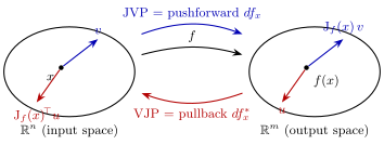
JVP (Jacobian–vector product).
\[\mathrm{J}_f(x)\, v = \begin{bmatrix} \nabla f_1(x)^\top \\ \vdots \\ \nabla f_m(x)^\top \end{bmatrix} v = \begin{bmatrix} \langle \nabla f_1(x), v \rangle \\ \vdots \\ \langle \nabla f_m(x), v \rangle \end{bmatrix} \simeq \frac{f(x + h v) - f(x)}{h}, \qquad h > 0.\] The finite-difference approximation uses two evaluations of \(f\), at \(x\) and \(x+hv\); forward-mode AD computes the JVP without a finite-difference step.
VJP (vector–Jacobian product).
For \(u\in\mathbb{R}^m\), the VJP is \(u^\top\mathrm{J}_f(x)\in\mathbb{R}^{1\times n}\). Applying forward differences to the scalar function \(x\mapsto u^\top f(x)\) uses \(n+1\) evaluations of \(f\); reverse-mode AD computes the VJP in one backward sweep.
The dual part \(\dot{x}\) (\(=b\) above) is a tangent vector,
so forward mode \(=\) JVP \(=\) pushforward, while reverse mode \(=\) VJP \(=\) pullback. This is the JAX mental model
(jvp/vjp):
6 Computational Graph
The key point to understand automatic differentiation is to view computer programs as evaluation of a computational graph. A computational graph represents the stack of evaluation performed by the program. Consider \(f : \mathbb{R}^n \to \mathbb{R}^m\) written as a composition \[o = f(x) = (f_4 \circ f_3 \circ f_2 \circ f_1)(x).\]

The intermediate variables are \[x_1 = x, \quad x_2 = f_1(x_1), \quad x_3 = f_2(x_2), \quad x_4 = f_3(x_3), \quad o = f_4(x_4).\] By the chain rule, \[\frac{\partial o}{\partial x} = \frac{\partial o}{\partial x_4}\, \frac{\partial x_4}{\partial x_3}\, \frac{\partial x_3}{\partial x_2}\, \frac{\partial x_2}{\partial x} = \mathrm{J}_{f_4}(x_4)\, \mathrm{J}_{f_3}(x_3)\, \big[\, \mathrm{J}_{f_2}(x_2)\, \mathrm{J}_{f_1}(x) \,\big].\] Writing \(f_1 : \mathbb{R}^n \to \mathbb{R}^{m_1}\), \(f_2 : \mathbb{R}^{m_1} \to \mathbb{R}^{m_2}\), \(f_3 : \mathbb{R}^{m_2} \to \mathbb{R}^{m_3}\) and \(f_4 : \mathbb{R}^{m_3} \to \mathbb{R}^m\), the order in which this product is evaluated determines the cost.
6.1 Forward mode
Since \(\mathrm{J}_f(x)\, e_j = \dfrac{\partial f}{\partial x_j}\), computing the full gradient \(\nabla f(x)\) (case \(m = 1\)) requires \(n\) JVPs, with cost \[n\big(m\, m_3 + m_3 m_2 + m_2 m_1 + m_1 n\big).\] For \(m = 1\) and \(m_1 = m_2 = m_3 = n\), this is \(O(n^3)\).
Algorithm: Forward mode
6.2 Reverse mode (backpropagation)
Since \(e_i^\top \mathrm{J}_f(x) = \nabla f_i(x)^\top\), computing a gradient (case \(m = 1\)) requires a single VJP, \[u^\top \mathrm{J}_{f_4}(x_4) \cdots \mathrm{J}_{f_1}(x),\] with cost \[m\big(m\, m_3 + m_3 m_2 + m_2 m_1 + m_1 n\big).\] For \(m = 1\) and \(m_1 = m_2 = m_3 = n\), this is \(O(n^2)\).
Reverse mode stores the intermediate values needed by the backward pass, using memory proportional to the total size of those stored values. Forward mode can stream through a chain, retaining only the current primal and tangent states. Checkpointing is a way to alleviate this issue.
Algorithm: Reverse mode
7 Backpropagation on a General Graph
The graph above was a chain: every node had exactly one predecessor, so the Jacobian factorised as a single sequential product. A real program is not a chain but a directed acyclic graph (DAG): a variable may feed several operations (fan-out) and an operation may read several variables (fan-in). The running example \(f(x_1, x_2) = x_1 + x_2 + x_1 x_2 + e^{x_1}\) is exactly of this kind – \(x_1\) is consumed three times.
The graph.
Write \(G = (V, E)\) for the DAG. Each non-source node \(v\) computes an elementary operation of its parents, \[x_v = \phi_v\big((x_u)_{u \in \mathrm{pa}(v)}\big),\] where \(\mathrm{pa}(v)\) denotes the parents of \(v\). The sources are the inputs \(x_1, \dots, x_n\), and we assume a single sink \(o\) (a scalar output; several outputs are handled by seeding several adjoints).
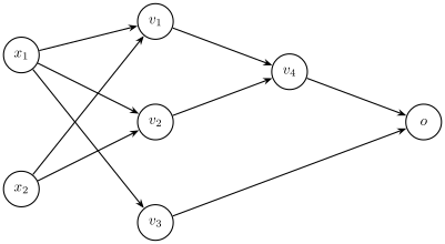
+ - * /, ^, exp/sin/cos/log/sqrt/tanh). Above each node: value (forward). Below, in colour: adjoint ∂o/∂· (reverse).with \[v_1 = x_1 + x_2, \quad v_2 = x_1 x_2, \quad v_3 = e^{x_1}, \quad v_4 = v_1 + v_2, \quad o = v_3 + v_4.\]
Topological order.
A topological order is a linear ordering \(v_1, \dots, v_N\) of \(V\) in which every node appears after all its parents; it exists if and only if \(G\) is acyclic. After assigning the inputs to the source nodes, evaluating the remaining nodes in this order – the forward pass – computes each \(x_v\) from already-available parents and reproduces \(o = f(x)\).
The chain rule with fan-out.
Let the adjoint of \(v\) be the (column) gradient of the output with respect to that node, \(\bar{x}_v = \nabla_{x_v} o\). Applying the chain rule at every operation that consumes \(x_v\), the adjoint accumulates one contribution per child: \[\boxed{\;\bar{x}_v = \sum_{w \,:\, v \to w} \Big(\frac{\partial \phi_w}{\partial x_v}\Big)^{\!\top} \bar{x}_w\;}\] This sum is the entire difference with the chain case. When every node has a single child the sum has one term and we recover the sequential product \(u^\top \mathrm{J}_{f_4} \cdots \mathrm{J}_{f_1}\) of the linear case above; fan-out is precisely what a chain cannot express, and the gradient of a reused variable is the sum of the contributions of all its uses.
Reverse sweep.
Seed \(\bar{x}_o = 1\) and visit the nodes in reverse topological order: this guarantees that when \(v\) is reached, the adjoints of all its children are already final. In practice one organizes this as a push (or scatter): initialise every \(\bar{x}_v = 0\), and as each node \(w\) is processed it adds \((\partial \phi_w / \partial x_u)^\top \bar{x}_w\) to the accumulator of each parent \(u\). Each elementary operation then only needs its local VJP – how to turn an output cotangent into input cotangents – while the graph wiring and the reverse order handle the global accumulation. The adjoints of the inputs are the gradient, \(\nabla f(x) = (\bar{x}_1, \dots, \bar{x}_n)\).
Algorithm: Reverse-mode AD on a DAG (backpropagation)
The example, backward.
The reverse sweep gives \(\bar{x}_o = 1\), then \(\bar{v}_4 = \bar{v}_3 = 1\) and \(\bar{v}_1 = \bar{v}_2 = 1\). The reused input \(x_1\), with the three children \(v_1, v_2, v_3\), collects three terms, \[\bar{x}_1 = \underbrace{1 \cdot \bar{v}_1}_{\text{via } +} + \underbrace{x_2 \cdot \bar{v}_2}_{\text{via } \times} + \underbrace{e^{x_1} \cdot \bar{v}_3}_{\text{via } \exp} = 1 + x_2 + e^{x_1}, \qquad \bar{x}_2 = 1 \cdot \bar{v}_1 + x_1 \cdot \bar{v}_2 = 1 + x_1,\] which is exactly \(\nabla f(x)\).
Cost.
Each edge is traversed once per pass, so the backward sweep costs a constant times the forward graph, the cheap-gradient principle on an arbitrary DAG, at the price of storing the intermediates \(x_v\) (the tape). A finite loop can be unrolled into an acyclic computation and differentiated by backpropagation. For an output defined by an implicit relation, such as a fixed point, implicit differentiation is another option.